데이터 사이언스 07 시계열 데이터 02-주가예측-prophet
1. 주가예측 - statsmodels
1) 모듈명 변경 및 설치
- 과거 pandas.io.data 모듈이
pandas_datareader.data로 바뀜 - 모듈 설치
➜  pip install pandas-datareader

Collecting pandas-datareader
  Downloading pandas_datareader-0.5.0-py2.py3-none-any.whl (74kB)
    100% |████████████████████████████████| 81kB 606kB/s
Installing collected packages: requests-ftp, requests-file, pandas-datareader
  Running setup.py install for requests-ftp ... done
Successfully installed pandas-datareader-0.5.0 requests-file-1.4.3 requests-ftp-0.3.1
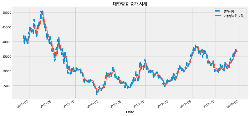
2) 대한항공 주가
- 종목 코드 : 003490
- 2015년 1월 1일부터 현재까지의 주가
import warnings
warnings.filterwarnings("ignore")

import itertools
import pandas as pd
import numpy as np

import statsmodels.api as sm
import matplotlib.pyplot as plt
plt.style.use('fivethirtyeight')
%matplotlib inline

# 한글폰트
import matplotlib.font_manager as fm
# 폰트 적용
font_location = '/usr/share/fonts/truetype/nanum/NanumBarunGothic.ttf'
font_name = fm.FontProperties(fname=font_location).get_name()

from matplotlib import rc
rc('font', family=font_name)
import pandas_datareader.data as web
from datetime import datetime
# 대한항공 2015. 1. 1.부터 현재까지의 주가

start = datetime( 2015, 1, 1 )
end = datetime.now()

# yahoo 파이낸스
KA = web.DataReader('003490.KS', 'yahoo', start, end)
KA.head()
| Open | High | Low | Close | Adj Close | Volume | |
|---|---|---|---|---|---|---|
| Date | ||||||
| 2015-01-02 | 43374.101563 | 44282.398438 | 40966.898438 | 41012.300781 | 41012.300781 | 1062595 |
| 2015-01-05 | 41330.300781 | 42329.500000 | 40194.800781 | 41966.101563 | 41966.101563 | 912246 |
| 2015-01-06 | 42374.898438 | 43192.398438 | 41466.500000 | 41466.500000 | 41466.500000 | 948055 |
| 2015-01-07 | 39059.398438 | 40558.199219 | 37197.199219 | 39513.601563 | 39513.601563 | 3256086 |
| 2015-01-08 | 39604.398438 | 40240.199219 | 38605.199219 | 39331.898438 | 39331.898438 | 549048 |
KA['Close'].plot(
    style='--',
    figsize=(12, 6)
)
pd.rolling_mean( KA['Close'], 7).plot( lw=2 )
plt.title('대한항공 종가 시세')
plt.legend( ['종가시세', '이동평균선(7일)' ] )
plt.show()
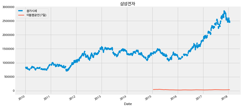
3) 삼성전자 주가
- 종목 코드: 005930
start = datetime( 2010, 1, 1 )
end = datetime.now()

SamSung = web.DataReader('005930.KS', 'yahoo', start, end)
SamSung['Close'].plot(
    style='--',
    figsize=(12, 6)
)
pd.rolling_mean( KA['Close'], 7).plot( lw=2 )
plt.title('삼성전자')
plt.legend( ['종가시세', '이동평균선(7일)' ] )
plt.show()
SamSung.head(3)
| Open | High | Low | Close | Adj Close | Volume | |
|---|---|---|---|---|---|---|
| Date | ||||||
| 2010-01-04 | 803000.0 | 809000.0 | 800000.0 | 809000.0 | 740499.0625 | 239016 |
| 2010-01-05 | 826000.0 | 829000.0 | 815000.0 | 822000.0 | 752398.2500 | 558517 |
| 2010-01-06 | 829000.0 | 841000.0 | 826000.0 | 841000.0 | 769789.5000 | 458977 |
len(SamSung)
1991
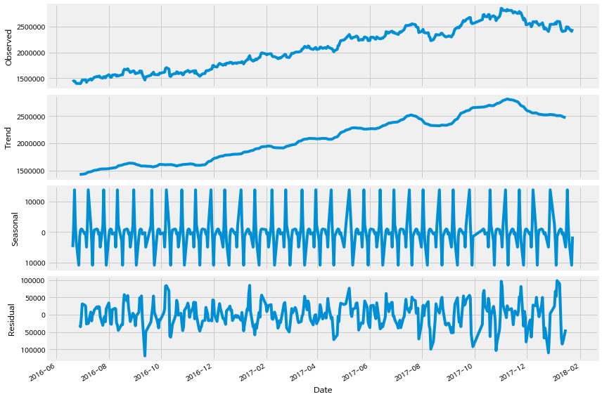
from pylab import rcParams
rcParams['figure.figsize'] = 12, 8

# 삼성전자 주식 종가에 대한 분해
y = SamSung['Close'][ 1600 : ]

decomposition = sm.tsa.seasonal_decompose(  y, freq=12 )

fig = decomposition.plot()
plt.show()
# Define the p, d and q parameters to take any value between 0 and 2
p = d = q = range(0, 2)

# Generate all different combinations of p, q and d triplets
pdq = list( itertools.product(p, d, q))

# Generate all different combinations of seasonal p, q and d triplets
seasonal_pdq = [ (x[0], x[1], x[2], 12)  for x in pdq ]

print('Example of parameter combinations for Seasonal ARIMA ...')
print('SARIMAX:  {} x {}'.format(pdq[1], seasonal_pdq[1]) )
print('SARIMAX:  {} x {}'.format(pdq[1], seasonal_pdq[2]) )
print('SARIMAX:  {} x {}'.format(pdq[2], seasonal_pdq[3]) )
print('SARIMAX:  {} x {}'.format(pdq[2], seasonal_pdq[4]) )
Example of parameter combinations for Seasonal ARIMA ...
SARIMAX:  (0, 0, 1) x (0, 0, 1, 12)
SARIMAX:  (0, 0, 1) x (0, 1, 0, 12)
SARIMAX:  (0, 1, 0) x (0, 1, 1, 12)
SARIMAX:  (0, 1, 0) x (1, 0, 0, 12)
warnings.filterwarnings("ignore")

y = SamSung['Close']

select_candi = 10000000
param_candi = ( 0, 0, 0 )
param_seasonal_candi = ( 0, 0, 0)

count=0
end_count = len(pdq)

for param in pdq:
    for param_seasonal in seasonal_pdq:
        try:
            mod = sm.tsa.statespace.SARIMAX(
                                            y,
                                            order=param,
                                            seasonal_order=param_seasonal,
                                            enforce_stationarity=False,
                                            enforce_invertibility=False
                                           )
            results = mod.fit()
            count += 1
            if count <= 5:
                print('ARIMA{}x{}12 - AIC:{}'.format(param, param_seasonal, results.aic))

            if results.aic < select_candi:
                select_candi = results.aic
                param_candi = param
                param_seasonal_candi = param_seasonal
        except:
            continue

print(param_candi, param_seasonal_candi, select_candi)
ARIMA(0, 0, 0)x(0, 0, 1, 12)12 - AIC:60253.297878071855
ARIMA(0, 0, 0)x(0, 1, 1, 12)12 - AIC:49644.270908598235
ARIMA(0, 0, 0)x(1, 0, 0, 12)12 - AIC:49928.79116493459
ARIMA(0, 0, 0)x(1, 0, 1, 12)12 - AIC:49903.76087716084
ARIMA(0, 0, 0)x(1, 1, 0, 12)12 - AIC:49669.749916549496
(1, 1, 1) (0, 0, 1, 12) 45391.1132768003
mod = sm.tsa.statespace.SARIMAX(
    y,
    order=(1, 1, 1),
    seasonal_order=(0, 0, 1, 12),
    enforce_stationarity=False,
    enforce_invertibility=False
)

results = mod.fit()

print( results.summary().tables[1] )
==============================================================================
                 coef    std err          z      P>|z|      [0.025      0.975]
------------------------------------------------------------------------------
ar.L1         -0.6241      0.182     -3.431      0.001      -0.981      -0.268
ma.L1          0.6733      0.172      3.925      0.000       0.337       1.010
ma.S.L12       0.0194      0.019      0.997      0.319      -0.019       0.058
sigma2      5.519e+08   5.22e-11   1.06e+19      0.000    5.52e+08    5.52e+08
==============================================================================
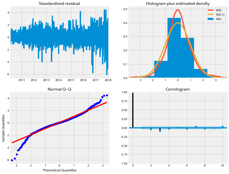
results.plot_diagnostics( figsize=(12, 10) )
plt.show()
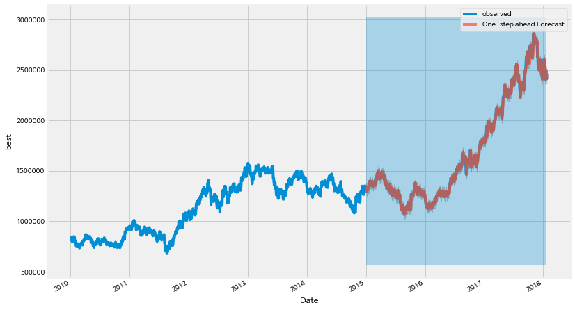
pred = results.get_prediction(
    start=pd.to_datetime('2015-1-2'),
    dynamic=False
)

pred_ci = pred.conf_int()
# 관측 데이터  1973년 부터 끝까지
ax = y[ '2000' : ].plot( label='observed', figsize=(12, 8) )

# 예측
pred.predicted_mean.plot(
    ax=ax,
    label='One-step ahead Forecast',
    alpha=.7
)

ax.fill_between(
    pred_ci.index,
    pred_ci.iloc[ : , 0 ],
    pred_ci.iloc[ : , 1 ],
    color='k',
    alpha=.2
)

ax.fill_betweenx(
    ax.get_ylim(),
    pd.to_datetime('2015-01-01'),
    y.index[-1],
    alpha=.3,
)

ax.set_xlabel('Date')
ax.set_ylabel('best')
plt.legend()

plt.show()
y = SamSung['Close'].resample('MS').mean()
warnings.filterwarnings("ignore")

select_candi = 10000000
param_candi = ( 0, 0, 0 )
param_seasonal_candi = ( 0, 0, 0)

count=0
end_count = len(pdq)

for param in pdq:
    for param_seasonal in seasonal_pdq:
        try:
            mod = sm.tsa.statespace.SARIMAX(
                                            y,
                                            order=param,
                                            seasonal_order=param_seasonal,
                                            enforce_stationarity=False,
                                            enforce_invertibility=False
                                           )
            results = mod.fit()
            count += 1
            if count <= 5:
                print('ARIMA{}x{}12 - AIC:{}'.format(param, param_seasonal, results.aic))

            if results.aic < select_candi:
                select_candi = results.aic
                param_candi = param
                param_seasonal_candi = param_seasonal
        except:
            continue

print(param_candi, param_seasonal_candi, select_candi)
ARIMA(0, 0, 0)x(0, 0, 1, 12)12 - AIC:2588.3600182104815
ARIMA(0, 0, 0)x(0, 1, 1, 12)12 - AIC:2077.9442515545934
ARIMA(0, 0, 0)x(1, 0, 0, 12)12 - AIC:2411.5750802284015
ARIMA(0, 0, 0)x(1, 0, 1, 12)12 - AIC:2388.3744838038806
ARIMA(0, 0, 0)x(1, 1, 0, 12)12 - AIC:2100.2859990842962
(0, 1, 1) (1, 1, 1, 12) 1798.848144371688
mod = sm.tsa.statespace.SARIMAX(
    y,
    order=( 0, 1, 1 ),
    seasonal_order=( 1, 1, 1, 12 ),
    enforce_stationarity=False,
    enforce_invertibility=False
)

results = mod.fit()

print( results.summary().tables[1] )
==============================================================================
                 coef    std err          z      P>|z|      [0.025      0.975]
------------------------------------------------------------------------------
ma.L1          0.2222      0.243      0.916      0.360      -0.253       0.698
ar.S.L12      -0.8107      0.208     -3.888      0.000      -1.219      -0.402
ma.S.L12      -0.0022      0.278     -0.008      0.994      -0.546       0.542
sigma2      1.145e+10   7.04e-12   1.63e+21      0.000    1.15e+10    1.15e+10
==============================================================================
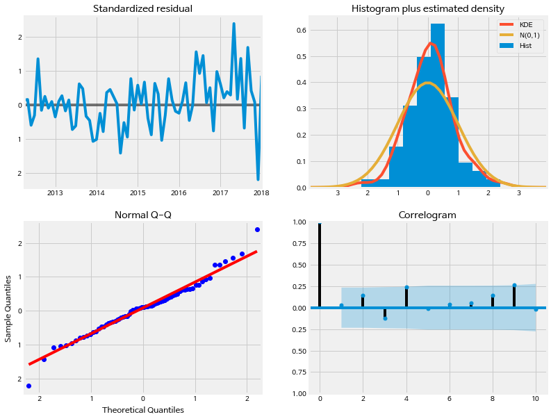
results.plot_diagnostics( figsize=(12, 10) )
plt.show()
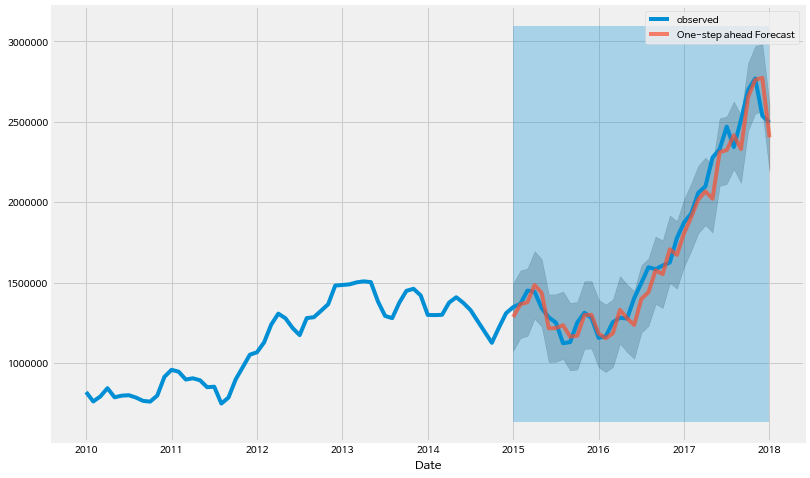
pred = results.get_prediction(
    start=pd.to_datetime('2015-01-01'),
    dynamic=False
)

pred_ci = pred.conf_int()
# 관측 데이터  2003년 부터 끝까지
ax = y[ '2003' : ].plot( label='observed', figsize=(12, 8) )

# 예측
pred.predicted_mean.plot(
    ax=ax,
    label='One-step ahead Forecast',
    alpha=.7
)

ax.fill_between(
    pred_ci.index,
    pred_ci.iloc[ : , 0 ],
    pred_ci.iloc[ : , 1 ],
    color='k',
    alpha=.2
)

ax.fill_betweenx(
    ax.get_ylim(),
    pd.to_datetime('2015-01-01'),
    y.index[-1],
    alpha=.3,
)

ax.set_xlabel('Date')
plt.legend()

plt.show()
2. 주가예측 - Prophet
https://facebook.github.io/prophet/
https://github.com/facebook/prophet
1) install
- Ubuntu16.04LTS, Python 3.6.2 환경
- 패키지로 설치하는 것이 편하고 안전하다.
➜  pip install fbprophet

Collecting fbprophet
  Downloading fbprophet-0.2.1.tar.gz
Collecting pystan>=2.14 (from fbprophet)
  Downloading pystan-2.17.1.0-cp36-cp36m-manylinux1_x86_64.whl (68.1MB)
  100% |████████████████████████████████| 68.1MB
  Downloading Cython-0.27.3-cp36-cp36m-manylinux1_x86_64.whl (3.1MB)
  100% |████████████████████████████████| 3.1MB 236kB/s
Installing collected packages: Cython, pystan, fbprophet
  Running setup.py install for fbprophet ... \
2) 기아자동차 주식
import warnings
warnings.filterwarnings("ignore")

import itertools
import pandas as pd
import numpy as np

import statsmodels.api as sm
import matplotlib.pyplot as plt
plt.style.use('fivethirtyeight')
%matplotlib inline
import pandas_datareader.data as web
from datetime import datetime

# 한글폰트
import matplotlib.font_manager as fm
# 폰트 적용
font_location = '/usr/share/fonts/truetype/nanum/NanumBarunGothic.ttf'
font_name = fm.FontProperties(fname=font_location).get_name()

from matplotlib import rc
rc('font', family=font_name)


from fbprophet import Prophet
start = datetime( 1990, 1, 1 )
end = datetime( 2017, 6, 30 )
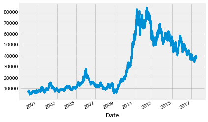
# 기아자동차 주식
KIA = web.DataReader('000270.KS', 'yahoo', start, end )
KIA.head()
| Open | High | Low | Close | Adj Close | Volume | |
|---|---|---|---|---|---|---|
| Date | ||||||
| 2000-01-04 | 7404.520020 | 7665.240234 | 7300.229980 | 7665.240234 | 6111.007324 | 636300.0 |
| 2000-01-05 | 7404.520020 | 7404.520020 | 7248.089844 | 7248.089844 | 5778.440918 | 686100.0 |
| 2000-01-06 | 7331.520020 | 7519.240234 | 6935.220215 | 6935.220215 | 5529.009277 | 379000.0 |
| 2000-01-07 | 6987.359863 | 7143.799805 | 6778.790039 | 6778.790039 | 5404.296875 | 701400.0 |
| 2000-01-10 | 6841.359863 | 7102.080078 | 6810.069824 | 7091.649902 | 5653.720703 | 1076700.0 |
KIA['Close'].plot()
<matplotlib.axes._subplots.AxesSubplot at 0x7f1f1d6a3160>
# 2016-12-31까지

KIA_trunc = KIA[ : '2016-12-31' ]
KIA_trunc.head(3)
| Open | High | Low | Close | Adj Close | Volume | |
|---|---|---|---|---|---|---|
| Date | ||||||
| 2000-01-04 | 7404.52002 | 7665.240234 | 7300.229980 | 7665.240234 | 6111.007324 | 636300.0 |
| 2000-01-05 | 7404.52002 | 7404.520020 | 7248.089844 | 7248.089844 | 5778.440918 | 686100.0 |
| 2000-01-06 | 7331.52002 | 7519.240234 | 6935.220215 | 6935.220215 | 5529.009277 | 379000.0 |
df = pd.DataFrame(
    {
        'ds': KIA_trunc.index,
        'y'  : KIA_trunc['Close']
    }
)

df.reset_index( inplace=True )
del df['Date']
df.head(3)
| ds | y | |
|---|---|---|
| 0 | 2000-01-04 | 7665.240234 |
| 1 | 2000-01-05 | 7248.089844 |
| 2 | 2000-01-06 | 6935.220215 |
m = Prophet()
m.fit(df)
<fbprophet.forecaster.Prophet at 0x7f1f1cb3a7f0>
future = m.make_future_dataframe( periods=365 )
future.tail(3)
| ds | |
|---|---|
| 4663 | 2017-12-27 |
| 4664 | 2017-12-28 |
| 4665 | 2017-12-29 |
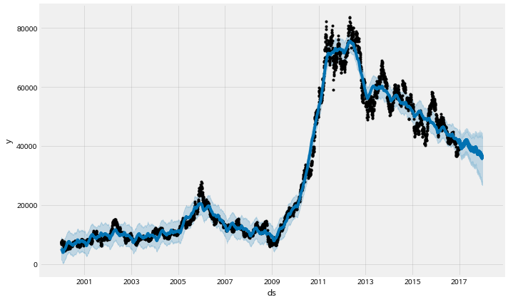
forecast = m.predict( future )
forecast[ [ 'ds', 'yhat', 'yhat_lower', 'yhat_upper' ] ].tail()
| ds | yhat | yhat_lower | yhat_upper | |
|---|---|---|---|---|
| 4661 | 2017-12-25 | 35736.021198 | 26901.256042 | 43506.681983 |
| 4662 | 2017-12-26 | 35781.066339 | 26897.317236 | 42529.643307 |
| 4663 | 2017-12-27 | 35749.136369 | 26619.638417 | 43537.664311 |
| 4664 | 2017-12-28 | 35714.091179 | 26785.438078 | 43183.694451 |
| 4665 | 2017-12-29 | 35650.791639 | 26849.725225 | 43201.114843 |
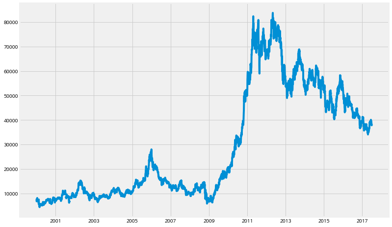
plt.figure( figsize=( 12, 8) )
plt.plot( KIA['Close'] )
plt.show()
m.plot(forecast)

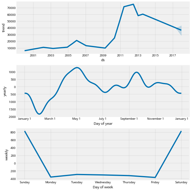
m.plot_components( forecast )

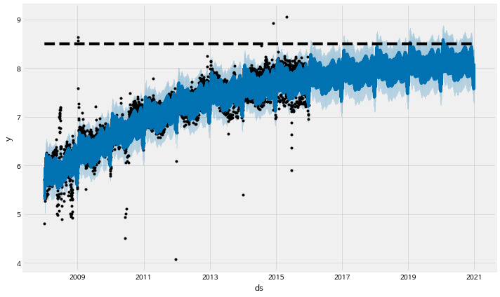
3) 기아자동차 주식 - Growth Model
df = pd.read_csv( './data_science/07. example_wp_R.csv' )
df['y' ] = np.log( df['y'] )
df['cap'] = 8.5
m = Prophet( growth='logistic' )
m.fit(df)
<fbprophet.forecaster.Prophet at 0x7f1f271417f0>
future = m.make_future_dataframe( periods=1826 )
future['cap'] = 8.5
fcst = m.predict( future )
m.plot( fcst )