데이터 사이언스 09 이미지 처리-mahotas

게시: January 23, 2018 by 주인장

주제별:
Data-Science 13

1. 참조
2. 모듈 설치 - mahotas
3. 경계 찾기
- 1) 흑백
- 2) 블러링
4. 초점 맞추기
5. 이미지 분류

1. 참조

Mahotas: Computer Vision in Python 공식문서

Image Processing in OpenCV

2. 모듈 설치 - mahotas

➜  pip install mahotas

Successfully installed mahotas-1.4.4

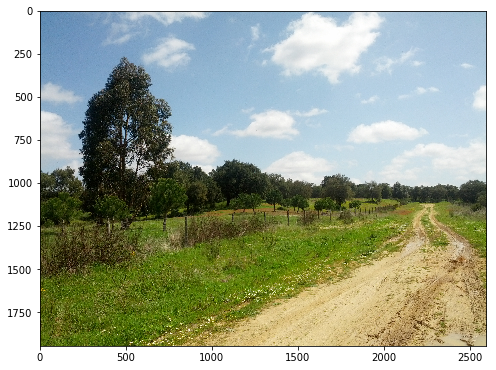
3. 경계 찾기

Canny Edge Detection

1) 흑백

import mahotas as mh
import numpy as np
from matplotlib import pyplot as plt
%matplotlib inline

image_raw = mh.imread( './data_science/scene06.jpg' )

plt.figure( figsize=(8, 8) )
plt.imshow(image_raw)
plt.show()

png

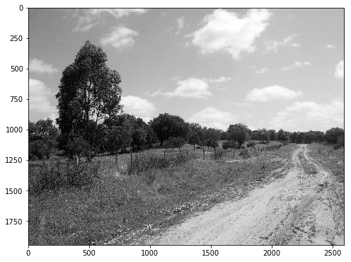
image_grey = mh.colors.rgb2grey( image_raw )

plt.figure( figsize=(8, 8) )
plt.imshow( image_grey )
plt.gray()
plt.show()

png

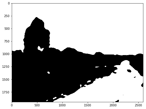
thresholding = mh.thresholding.otsu( image )
print( 'Otsu threshold is {}'.format(thresholding))

Otsu threshold is 128

plt.figure( figsize=(8, 8))
plt.imshow( image_grey>thresholding )
plt.show()

png

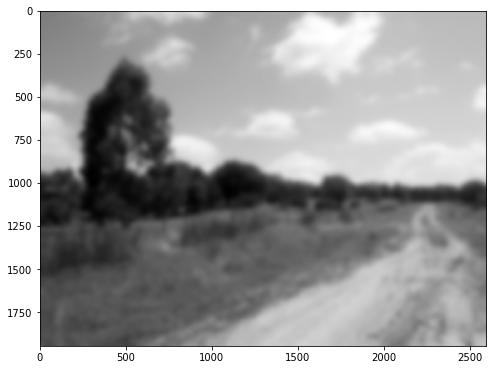
2) 블러링

# 가우시안 블러링

im16 = mh.gaussian_filter( image_grey, 16 )

/home/learn/.pyenv/versions/3.6.2/envs/Jupyter/lib/python3.6/site-packages/mahotas/internal.py:112: FutureWarning: Conversion of the second argument of issubdtype from `float` to `np.floating` is deprecated. In future, it will be treated as `np.float64 == np.dtype(float).type`.
  if not np.issubdtype(A.dtype, np.float):

plt.figure(figsize=(8,8))
plt.imshow(im16)
plt.show()

png

plt.figure(figsize=(8,8))
plt.imshow( im16>thresholding )
plt.show()

png

4. 초점 맞추기

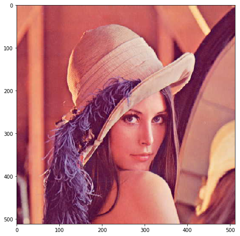
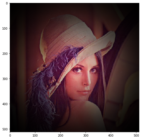
lena_raw = mh.demos.load('lena')

plt.figure(figsize=(8, 8))
plt.imshow(lena_raw)
plt.show()

png

test_transpose_origin = np.array(
    [
        [ [1, 2], [3, 4], [5, 6] ],
        [ [7, 8], [9, 10], [11, 12] ],
        [ [13,14], [15,16], [17,18] ]
    ]
)
print( test_transpose_origin.shape)
print( test_transpose_origin)

(3, 3, 2)
[[[ 1  2]
  [ 3  4]
  [ 5  6]]

 [[ 7  8]
  [ 9 10]
  [11 12]]

 [[13 14]
  [15 16]
  [17 18]]]

test_transpose = test_transpose_origin.transpose(2, 0, 1)
print( test_transpose )

[[[ 1  3  5]
  [ 7  9 11]
  [13 15 17]]

 [[ 2  4  6]
  [ 8 10 12]
  [14 16 18]]]

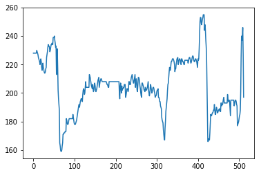
r, g, b = lena_raw.transpose(2, 0, 1)

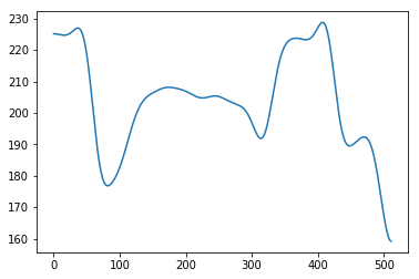
r12 = mh.gaussian_filter( r, 12.)
g12 = mh.gaussian_filter( g, 12.)
b12 = mh.gaussian_filter( b, 12.)

im12 = mh.as_rgb(r12, g12, b12)

/home/learn/.pyenv/versions/3.6.2/envs/Jupyter/lib/python3.6/site-packages/mahotas/internal.py:112: FutureWarning: Conversion of the second argument of issubdtype from `float` to `np.floating` is deprecated. In future, it will be treated as `np.float64 == np.dtype(float).type`.
  if not np.issubdtype(A.dtype, np.float):

plt.plot( r[0] )
plt.show()

png

plt.plot( r12[0] )
plt.show()

png

h, w = r.shape
Y, X = np.mgrid[ :h, :w ]

Y = Y - h/2.
Y = Y / Y.max()

X = X - h/2.
X = X / X.max()

C = np.exp( -2.*( X**2 + Y**2 ) )

C = C - C.min()
C = C / C.ptp()
C.shape

(512, 512)

C = C[:, :, None ]
C.shape

(512, 512, 1)

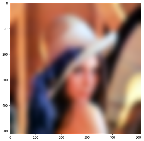
# 중앙 초점

ringed = mh.stretch(lena_raw*C)

plt.figure( figsize=(8,8) )
plt.imshow(ringed)
plt.show()

png

plt.figure( figsize=(8, 8))
plt.imshow( im12 )
plt.show()

png

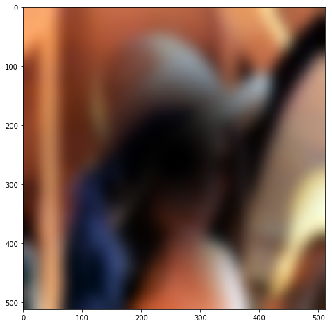
ringed = mh.stretch( (1-C)*im12 )

plt.figure( figsize=(8,8) )
plt.imshow(ringed)
plt.show()

png

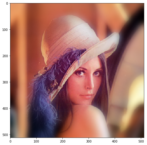
ringed = mh.stretch( lena_raw*C + (1 - C)*im12)

plt.figure( figsize=(8,8) )
plt.imshow(ringed)
plt.show()

png

5. 이미지 분류

scikit-learn 공식문서

1) scikit-learn 설치

➜  pip install -U scikit-learn


Installing collected packages: scikit-learn
Successfully installed scikit-learn-0.19.1

2) 이미지 모음

from glob import glob

images = glob('./data_science/SimpleImageDataset/*.jpg')

images[:5]

['./data_science/SimpleImageDataset/text14.jpg',
 './data_science/SimpleImageDataset/building04.jpg',
 './data_science/SimpleImageDataset/scene04.jpg',
 './data_science/SimpleImageDataset/scene05.jpg',
 './data_science/SimpleImageDataset/text24.jpg']

images[0][ len("./data_science/SimpleImageDataset/") : - len('00.jpg')]

'text'

im = mh.imread( images[0] )

im = mh.colors.rgb2gray( im, dtype=np.uint8)

3) 이미지 특성(haralick 방법)과 라벨을 추출

features = []
labels = []
for im in images:
    labels.append( im[ len("./data_science/SimpleImageDataset/") : - len('00.jpg')] )
    im = mh.imread(im)
    im = mh.colors.rgb2gray( im, dtype=np.uint8 )
    features.append( mh.features.haralick(im).ravel() )

from sklearn.pipeline import Pipeline
from sklearn.preprocessing import StandardScaler
from sklearn.linear_model import LogisticRegression
# from sklearn import cross_validation
from sklearn import model_selection 

clf = Pipeline(
    [
        ( 'preproc', StandardScaler()), 
        ( 'classifier', LogisticRegression() )
    ]
)

cv = model_selection.LeaveOneOut( )
cv.get_n_splits( images )

scores = model_selection.cross_val_score( clf, features, labels, cv=cv )
scores

array([1., 0., 1., 0., 1., 1., 1., 1., 1., 1., 0., 1., 1., 1., 1., 0., 1.,
       1., 1., 0., 1., 1., 1., 1., 1., 1., 1., 1., 1., 1., 1., 1., 1., 1.,
       1., 1., 0., 1., 1., 1., 1., 1., 1., 1., 1., 0., 1., 0., 1., 1., 0.,
       1., 0., 1., 0., 1., 1., 1., 1., 1., 1., 0., 1., 1., 1., 1., 0., 1.,
       1., 1., 1., 1., 0., 1., 1., 0., 1., 1., 1., 1., 1., 0., 1., 1., 1.,
       1., 1., 1., 0., 1.])

print( 'Accuracy:  {: .2%}'.format( scores.mean() ) )

Accuracy:   81.11%

def chist(im):
    """Compute color histograms of input image
    Parameters
    ----------------------
    im  :  ndarray
            should be an RGB image
    Returns
    ---------------
    c  :  ndarray
           1-D array of histogram values
    """    
    # Downsample pixel values
    im = im//64
    # We can also implement the following by using np.histogramdd
    # im = im.reshape((-1, 3))
    # bins = [ np.arange(5),  np.arange(5),  np.arange(5) ]
    # hist = np.histogramdd( im, bins=bins )[0]
    # hist = hist.ravel()
    
    # Separate RGB channels
    r, g, b = im.transpose( (2, 0, 1) )
    
    pixels = 1*r + 4*g + 16*b
    hist = np.bincount( pixels.ravel(), minlength=64 )
    hist = hist.astype(float)
    return np.log1p(hist)    

features = []
for im in images:
    image = mh.imread(im)
    features.append( chist(image) )

scores = model_selection.cross_val_score( clf, features, labels, cv=cv )
print( 'Accuracy:  {: .2%}'.format( scores.mean() ) )

Accuracy:   91.11%

# 모든 속성을 반영

features = []
for im in images:
    imcolor = mh.imread(im)
    im = mh.colors.rgb2gray( imcolor, dtype=np.uint8 )
    features.append(
        np.concatenate(
            [ mh.features.haralick(im).ravel(),  chist(imcolor), ]
        )
    )

scores = model_selection.cross_val_score( clf, features, labels, cv=cv )
print( 'Accuracy:  {: .2%}'.format( scores.mean() ) )

Accuracy:   96.67%

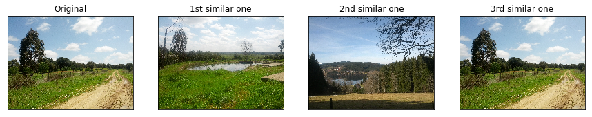
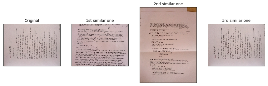
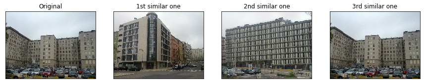
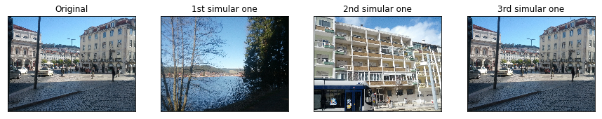
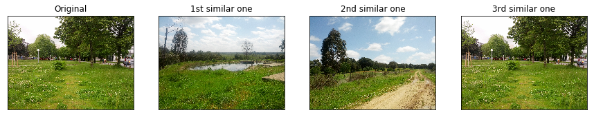
4) 유사 이미지 찾기

features = []
for im in images:
    imcolor = mh.imread(im)
    # Ignore everything in the 200 pixels close to the border
    imcolor = imcolor[200:-200, 200:-200]
    im = mh.colors.rgb2gray( imcolor, dtype=np.uint8 )
    features.append(
        np.concatenate(
            [ mh.features.haralick(im).ravel(),  chist(imcolor), ]
        )
    )

sc = StandardScaler()
features = sc.fit_transform(features)

from scipy.spatial  import distance

dists = distance.squareform( distance.pdist( features ) )

def selectImage( n, m, dists, images):
    image_position = dists[n].argsort()[m]
    image = mh.imread( images[image_position] )
    return image

def plotImages(n):
    plt.figure(figsize=(15, 15))
    
    plt.subplot(141)
    plt.imshow( selectImage(n, 0, dists, images) )
    plt.title('Original')
    plt.xticks([])
    plt.yticks([])
    
    plt.subplot(142)
    plt.imshow( selectImage(n, 1, dists, images) )
    plt.title('1st similar one')
    plt.xticks([])
    plt.yticks([])
    
    plt.subplot(143)
    plt.imshow( selectImage(n, 2, dists, images) )
    plt.title('2nd similar one')
    plt.xticks([])
    plt.yticks([])
    
    plt.subplot(144)
    plt.imshow( selectImage(n, 0, dists, images) )
    plt.title('3rd similar one')
    plt.xticks([])
    plt.yticks([])
    
    plt.show()

plotImages(0)

png

plotImages(1)

png

plotImages(11)

png

plotImages(31)

png

plotImages(61)

png