데이터 사이언스 01 주장의 근거- 서울시 CCTV
- 참조
- 1. 데이터 얻기
- 2. 서울시 구별 CCTV 현황 및 구별 인구 데이터 읽기
- ❈ pandas tutorials
- 3. 인구별 CCTV 비율을 확인하기
- 4. 인구대비 각 구별 CCTV 현황에 대한 경향 파악
- 5. 시각화
참조
1. 데이터 얻기
1) 서울시 구별 CCTV 현황
- 서울 열린데이터 광장 http://data.seoul.go.kr/
서울시 자치구 년도별 CCTV 설치 현황.csv➜01.CCTV_in_Seoul.csv
2) 서울시 구별 인구현황 데이터
- 서울 통계 http://stat.seoul.go.kr/
- 인구 > 주민등록인구 > 주민등록인구(구별)
OctagonExcel.xls➜01.population_in_Seoul.xls
2. 서울시 구별 CCTV 현황 및 구별 인구 데이터 읽기
1) pandas (powerful Python data analysis toolkit) 설치
$ pip install pandas

Collecting pandas
  Downloading pandas-0.22.0-cp36-cp36m-manylinux1_x86_64.whl (26.2MB)
    100% |████████████████████████████████| 26.3MB 34kB/s
Collecting numpy>=1.9.0 (from pandas)
  Using cached numpy-1.13.3-cp36-cp36m-manylinux1_x86_64.whl
Requirement already satisfied: python-dateutil>=2 in /home/learn/.pyenv/versions/3.6.2/envs/Jupyter/lib/python3.6/site-packages (from pandas)
Collecting pytz>=2011k (from pandas)
  Using cached pytz-2017.3-py2.py3-none-any.whl
Requirement already satisfied: six>=1.5 in /home/learn/.pyenv/versions/3.6.2/envs/Jupyter/lib/python3.6/site-packages (from python-dateutil>=2->pandas)
Installing collected packages: numpy, pytz, pandas
Successfully installed numpy-1.13.3 pandas-0.22.0 pytz-2017.3
2) 서울시 CCTV 데이터 읽기
import pandas as pd
CCTV_Seoul = pd.read_csv('./data_science/01.CCTV_in_Seoul.csv', encoding='utf-8')
CCTV_Seoul.head()
| 기관명 | 소계 | 2013년도 이전 | 2014년 | 2015년 | 2016년 | |
|---|---|---|---|---|---|---|
| 0 | 강남구 | 3238 | 1292 | 430 | 584 | 932 |
| 1 | 강동구 | 1010 | 379 | 99 | 155 | 377 |
| 2 | 강북구 | 831 | 369 | 120 | 138 | 204 |
| 3 | 강서구 | 911 | 388 | 258 | 184 | 81 |
| 4 | 관악구 | 2109 | 846 | 260 | 390 | 613 |
# 기관명  이름 (columns) 바꾸기
CCTV_Seoul.columns[0]
'기관명'
CCTV_Seoul.rename( columns={ CCTV_Seoul.columns[0] : '구별'}, inplace=True )
CCTV_Seoul.head()
| 구별 | 소계 | 2013년도 이전 | 2014년 | 2015년 | 2016년 | |
|---|---|---|---|---|---|---|
| 0 | 강남구 | 3238 | 1292 | 430 | 584 | 932 |
| 1 | 강동구 | 1010 | 379 | 99 | 155 | 377 |
| 2 | 강북구 | 831 | 369 | 120 | 138 | 204 |
| 3 | 강서구 | 911 | 388 | 258 | 184 | 81 |
| 4 | 관악구 | 2109 | 846 | 260 | 390 | 613 |
3) 서울시 인구현황 데이터 읽기
- 엑셀 읽는데 문제 발생
pop_Seoul = pd.read_excel('./data_science/01.population_in_Seoul.xls', encoding='utf-8')
ModuleNotFoundError: No module named 'xlrd'
- xlrd 설치
$ pip install xlrd

Collecting xlrd
  Downloading xlrd-1.1.0-py2.py3-none-any.whl (108kB)
    100% |████████████████████████████████| 112kB 670kB/s
Installing collected packages: xlrd
Successfully installed xlrd-1.1.0
pop_Seoul = pd.read_excel('./data_science/01.population_in_Seoul.xls', encoding='utf-8')
pop_Seoul.head()
| 기간 | 자치구 | 세대 | 인구 | 인구.1 | 인구.2 | 인구.3 | 인구.4 | 인구.5 | 인구.6 | 인구.7 | 인구.8 | 세대당인구 | 65세이상고령자 | |
|---|---|---|---|---|---|---|---|---|---|---|---|---|---|---|
| 0 | 기간 | 자치구 | 세대 | 합계 | 합계 | 합계 | 한국인 | 한국인 | 한국인 | 등록외국인 | 등록외국인 | 등록외국인 | 세대당인구 | 65세이상고령자 |
| 1 | 기간 | 자치구 | 세대 | 계 | 남자 | 여자 | 계 | 남자 | 여자 | 계 | 남자 | 여자 | 세대당인구 | 65세이상고령자 |
| 2 | 2017.3/4 | 합계 | 4219001 | 10158411 | 4975437 | 5182974 | 9891448 | 4849195 | 5042253 | 266963 | 126242 | 140721 | 2.34 | 1353486 |
| 3 | 2017.3/4 | 종로구 | 73668 | 164640 | 80173 | 84467 | 155109 | 76155 | 78954 | 9531 | 4018 | 5513 | 2.11 | 26034 |
| 4 | 2017.3/4 | 중구 | 60130 | 134174 | 66064 | 68110 | 125332 | 62011 | 63321 | 8842 | 4053 | 4789 | 2.08 | 21249 |
# 복잡한 header를 정리하기
##  header는 2번째 줄부터
##  사용할 coloumn은  B, D, G, J, N
##  FutureWarning: the 'parse_cols' keyword is deprecated, use 'usecols' instead
pop_Seoul = pd.read_excel(
                         './data_science/01.population_in_Seoul.xls',
                         header=2,
                         usecols='B, D, G, J, N',
                         encoding='utf-8'
                         )
pop_Seoul.head()
| 자치구 | 계 | 계.1 | 계.2 | 65세이상고령자 | |
|---|---|---|---|---|---|
| 0 | 합계 | 10158411.0 | 9891448.0 | 266963.0 | 1353486.0 |
| 1 | 종로구 | 164640.0 | 155109.0 | 9531.0 | 26034.0 |
| 2 | 중구 | 134174.0 | 125332.0 | 8842.0 | 21249.0 |
| 3 | 용산구 | 243922.0 | 228960.0 | 14962.0 | 36727.0 |
| 4 | 성동구 | 312933.0 | 304879.0 | 8054.0 | 40902.0 |
# Column 이름을 바꾸기
pop_Seoul.rename(
    columns={
        pop_Seoul.columns[0] : '구별',
        pop_Seoul.columns[1] : '인구수',
        pop_Seoul.columns[2] : '한국인',
        pop_Seoul.columns[3] : '외국인',
        pop_Seoul.columns[4] : '고령자'
    },
    inplace=True
)

pop_Seoul.head()
| 구별 | 인구수 | 한국인 | 외국인 | 고령자 | |
|---|---|---|---|---|---|
| 0 | 합계 | 10158411.0 | 9891448.0 | 266963.0 | 1353486.0 |
| 1 | 종로구 | 164640.0 | 155109.0 | 9531.0 | 26034.0 |
| 2 | 중구 | 134174.0 | 125332.0 | 8842.0 | 21249.0 |
| 3 | 용산구 | 243922.0 | 228960.0 | 14962.0 | 36727.0 |
| 4 | 성동구 | 312933.0 | 304879.0 | 8054.0 | 40902.0 |
import numpy as np
❈ pandas tutorials
1) pandas.Series( [배열] )
- input: 배열
- output: columns화
pandas.Series([1, 3, 5, numpy.nan, 6.8])

0    1.0
1    3.0
2    5.0
3    NaN
4    6.8
dtype:  float64
2) pandas.date_range( '일시', period=기간)
- Pandas는 시계열 데이터 처리에 강점을 가진다.
pandas.date_range('20130101', periods=6)

DatetimeIndex(['2013-01-01', '2013-01-02', '2013-01-03', '2013-01-04',
               '2013-01-05', '2013-01-06'],
              dtype='datetime64[ns]', freq='D')
3) pandas.DataFrame( index=배열1, columns=배열2)
- Pandas에서 가장 많이 사용하는 형태
- index가 행렬의 행(row)에 해당한다.
- pandas.DataFrame.index
- pandas.DataFrame.columns
- pandas.DataFrame.values
- pandas.DataFrame.**info() **
- pandas.DataFrame.describe()
- pandas.DataFrame.sort_values(by='컬럼명', ascending='True/False')
- pandas.DataFrame['칼럼이름']
pandas.DataFrame['A'] - pandas.DataFrame[인덱스 범위 n : m]
pandas.DataFrame[0 : 3] - pandas.DataFrame.loc['인덱스 번호']
pandas.DataFrame.loc['2013-01-01'] - pandas.DataFrame.loc[ i : j , [ m : n ] ]
pandas.DataFrame.loc[ '20130101' : '20130104', ['A', 'B'] ] - pandas.DataFrame.iloc[ i : j , [ m : n ] ]
- 조건부 슬라이싱
df[ df.A > 0 ],df[ df > 0 ]여기서df = pandas.DataFrame(행렬, index, columns) - DataFrame 복사
df2 = df.copy() - pandas.DataFrame.apply(함수)
df.apply(lambda x: x.max() - x.min() ) - 조건판단
df[df['E'].isin(['two', 'four'])
# CCTV 숫자가 적은 순으로 구별 정리
CCTV_Seoul.sort_values( by='소계', ascending=True).head()
| 구별 | 소계 | 2013년도 이전 | 2014년 | 2015년 | 2016년 | |
|---|---|---|---|---|---|---|
| 9 | 도봉구 | 825 | 238 | 159 | 42 | 386 |
| 2 | 강북구 | 831 | 369 | 120 | 138 | 204 |
| 5 | 광진구 | 878 | 573 | 78 | 53 | 174 |
| 3 | 강서구 | 911 | 388 | 258 | 184 | 81 |
| 24 | 중랑구 | 916 | 509 | 121 | 177 | 109 |
# CCTV 숫자가 많은 순으로 구별 정리
CCTV_Seoul.sort_values( by='소계', ascending=False).head()
| 구별 | 소계 | 2013년도 이전 | 2014년 | 2015년 | 2016년 | |
|---|---|---|---|---|---|---|
| 0 | 강남구 | 3238 | 1292 | 430 | 584 | 932 |
| 18 | 양천구 | 2482 | 1843 | 142 | 30 | 467 |
| 14 | 서초구 | 2297 | 1406 | 157 | 336 | 398 |
| 4 | 관악구 | 2109 | 846 | 260 | 390 | 613 |
| 21 | 은평구 | 2108 | 1138 | 224 | 278 | 468 |
CCTV_Seoul['최근증가율'] = \
( CCTV_Seoul['2016년'] + CCTV_Seoul['2015년'] + CCTV_Seoul['2014년'] ) / CCTV_Seoul['2013년도 이전'] * 100

CCTV_Seoul.sort_values(by='최근증가율', ascending=False).head()
| 구별 | 소계 | 2013년도 이전 | 2014년 | 2015년 | 2016년 | 최근증가율 | |
|---|---|---|---|---|---|---|---|
| 22 | 종로구 | 1619 | 464 | 314 | 211 | 630 | 248.922414 |
| 9 | 도봉구 | 825 | 238 | 159 | 42 | 386 | 246.638655 |
| 12 | 마포구 | 980 | 314 | 118 | 169 | 379 | 212.101911 |
| 8 | 노원구 | 1566 | 542 | 57 | 451 | 516 | 188.929889 |
| 1 | 강동구 | 1010 | 379 | 99 | 155 | 377 | 166.490765 |
4) 서울시 인구 데이터 정리하기
pop_Seoul.head()
| 구별 | 인구수 | 한국인 | 외국인 | 고령자 | |
|---|---|---|---|---|---|
| 0 | 합계 | 10158411.0 | 9891448.0 | 266963.0 | 1353486.0 |
| 1 | 종로구 | 164640.0 | 155109.0 | 9531.0 | 26034.0 |
| 2 | 중구 | 134174.0 | 125332.0 | 8842.0 | 21249.0 |
| 3 | 용산구 | 243922.0 | 228960.0 | 14962.0 | 36727.0 |
| 4 | 성동구 | 312933.0 | 304879.0 | 8054.0 | 40902.0 |
# '합계' 줄 제거
pop_Seoul.drop([0], inplace=True )
pop_Seoul.head()
| 구별 | 인구수 | 한국인 | 외국인 | 고령자 | |
|---|---|---|---|---|---|
| 1 | 종로구 | 164640.0 | 155109.0 | 9531.0 | 26034.0 |
| 2 | 중구 | 134174.0 | 125332.0 | 8842.0 | 21249.0 |
| 3 | 용산구 | 243922.0 | 228960.0 | 14962.0 | 36727.0 |
| 4 | 성동구 | 312933.0 | 304879.0 | 8054.0 | 40902.0 |
| 5 | 광진구 | 372414.0 | 357743.0 | 14671.0 | 43579.0 |
# '구별' 데이터 무결성 확인
pop_Seoul['구별'].unique()
array(['종로구', '중구', '용산구', '성동구', '광진구', '동대문구', '중랑구', '성북구', '강북구',
       '도봉구', '노원구', '은평구', '서대문구', '마포구', '양천구', '강서구', '구로구', '금천구',
       '영등포구', '동작구', '관악구', '서초구', '강남구', '송파구', '강동구', nan], dtype=object)
# nan 부분 확인
pop_Seoul[pop_Seoul['구별'].isnull()]
| 구별 | 인구수 | 한국인 | 외국인 | 고령자 | |
|---|---|---|---|---|---|
| 26 | NaN | NaN | NaN | NaN | NaN |
# nan이 들어간 행을 drop으로 삭제하자.
pop_Seoul.drop([26], inplace=True)
pop_Seoul.tail()
| 구별 | 인구수 | 한국인 | 외국인 | 고령자 | |
|---|---|---|---|---|---|
| 21 | 관악구 | 522849.0 | 505188.0 | 17661.0 | 69486.0 |
| 22 | 서초구 | 447177.0 | 442833.0 | 4344.0 | 52738.0 |
| 23 | 강남구 | 565731.0 | 560827.0 | 4904.0 | 64579.0 |
| 24 | 송파구 | 668366.0 | 661750.0 | 6616.0 | 75301.0 |
| 25 | 강동구 | 446760.0 | 442654.0 | 4106.0 | 55902.0 |
pop_Seoul['외국인비율'] = pop_Seoul['외국인'] / pop_Seoul['인구수'] * 100
pop_Seoul['고령자비율'] = pop_Seoul['고령자'] / pop_Seoul['인구수'] * 100
pop_Seoul.head()
| 구별 | 인구수 | 한국인 | 외국인 | 고령자 | 외국인비율 | 고령자비율 | |
|---|---|---|---|---|---|---|---|
| 1 | 종로구 | 164640.0 | 155109.0 | 9531.0 | 26034.0 | 5.788994 | 15.812682 |
| 2 | 중구 | 134174.0 | 125332.0 | 8842.0 | 21249.0 | 6.589950 | 15.836898 |
| 3 | 용산구 | 243922.0 | 228960.0 | 14962.0 | 36727.0 | 6.133928 | 15.056862 |
| 4 | 성동구 | 312933.0 | 304879.0 | 8054.0 | 40902.0 | 2.573714 | 13.070529 |
| 5 | 광진구 | 372414.0 | 357743.0 | 14671.0 | 43579.0 | 3.939433 | 11.701762 |
# 인구수가 많은 순으로  정렬
pop_Seoul.sort_values(by='인구수', ascending=False).head()
| 구별 | 인구수 | 한국인 | 외국인 | 고령자 | 외국인비율 | 고령자비율 | |
|---|---|---|---|---|---|---|---|
| 24 | 송파구 | 668366.0 | 661750.0 | 6616.0 | 75301.0 | 0.989877 | 11.266432 |
| 16 | 강서구 | 607877.0 | 601391.0 | 6486.0 | 75046.0 | 1.066992 | 12.345590 |
| 23 | 강남구 | 565731.0 | 560827.0 | 4904.0 | 64579.0 | 0.866843 | 11.415143 |
| 11 | 노원구 | 562278.0 | 558432.0 | 3846.0 | 73588.0 | 0.684003 | 13.087476 |
| 21 | 관악구 | 522849.0 | 505188.0 | 17661.0 | 69486.0 | 3.377839 | 13.289879 |
# 외국인 숫자 순으로 정렬
pop_Seoul.sort_values(by='외국인', ascending=False).head()
| 구별 | 인구수 | 한국인 | 외국인 | 고령자 | 외국인비율 | 고령자비율 | |
|---|---|---|---|---|---|---|---|
| 19 | 영등포구 | 401908.0 | 368818.0 | 33090.0 | 53620.0 | 8.233228 | 13.341362 |
| 17 | 구로구 | 443288.0 | 412972.0 | 30316.0 | 58260.0 | 6.838895 | 13.142697 |
| 18 | 금천구 | 253646.0 | 235608.0 | 18038.0 | 33818.0 | 7.111486 | 13.332755 |
| 21 | 관악구 | 522849.0 | 505188.0 | 17661.0 | 69486.0 | 3.377839 | 13.289879 |
| 6 | 동대문구 | 367769.0 | 352011.0 | 15758.0 | 55287.0 | 4.284755 | 15.033078 |
# 외국인 비율 순으로 정렬
pop_Seoul.sort_values(by='외국인비율', ascending=False).head()
| 구별 | 인구수 | 한국인 | 외국인 | 고령자 | 외국인비율 | 고령자비율 | |
|---|---|---|---|---|---|---|---|
| 19 | 영등포구 | 401908.0 | 368818.0 | 33090.0 | 53620.0 | 8.233228 | 13.341362 |
| 18 | 금천구 | 253646.0 | 235608.0 | 18038.0 | 33818.0 | 7.111486 | 13.332755 |
| 17 | 구로구 | 443288.0 | 412972.0 | 30316.0 | 58260.0 | 6.838895 | 13.142697 |
| 2 | 중구 | 134174.0 | 125332.0 | 8842.0 | 21249.0 | 6.589950 | 15.836898 |
| 3 | 용산구 | 243922.0 | 228960.0 | 14962.0 | 36727.0 | 6.133928 | 15.056862 |
# 고령자 숫자 순으로 정렬
pop_Seoul.sort_values(by='고령자', ascending=False).head()
| 구별 | 인구수 | 한국인 | 외국인 | 고령자 | 외국인비율 | 고령자비율 | |
|---|---|---|---|---|---|---|---|
| 24 | 송파구 | 668366.0 | 661750.0 | 6616.0 | 75301.0 | 0.989877 | 11.266432 |
| 16 | 강서구 | 607877.0 | 601391.0 | 6486.0 | 75046.0 | 1.066992 | 12.345590 |
| 12 | 은평구 | 491899.0 | 487507.0 | 4392.0 | 73850.0 | 0.892866 | 15.013245 |
| 11 | 노원구 | 562278.0 | 558432.0 | 3846.0 | 73588.0 | 0.684003 | 13.087476 |
| 21 | 관악구 | 522849.0 | 505188.0 | 17661.0 | 69486.0 | 3.377839 | 13.289879 |
# 고령자 비율 순으로 정렬
pop_Seoul.sort_values(by='고령자비율', ascending=False).head()
| 구별 | 인구수 | 한국인 | 외국인 | 고령자 | 외국인비율 | 고령자비율 | |
|---|---|---|---|---|---|---|---|
| 9 | 강북구 | 329042.0 | 325552.0 | 3490.0 | 56078.0 | 1.060655 | 17.042809 |
| 2 | 중구 | 134174.0 | 125332.0 | 8842.0 | 21249.0 | 6.589950 | 15.836898 |
| 1 | 종로구 | 164640.0 | 155109.0 | 9531.0 | 26034.0 | 5.788994 | 15.812682 |
| 10 | 도봉구 | 347338.0 | 345293.0 | 2045.0 | 52909.0 | 0.588764 | 15.232713 |
| 3 | 용산구 | 243922.0 | 228960.0 | 14962.0 | 36727.0 | 6.133928 | 15.056862 |
3. 인구별 CCTV 비율을 확인하기
1) CCTV 데이터와 인구현황 데이터를 병합하기
- 2017년 CCTV 개수만 살펴보기로 함
- 그래프를 대비함
data_result = pd.merge(CCTV_Seoul, pop_Seoul, on='구별')
data_result.head()
| 구별 | 소계 | 2013년도 이전 | 2014년 | 2015년 | 2016년 | 최근증가율 | 인구수 | 한국인 | 외국인 | 고령자 | 외국인비율 | 고령자비율 | |
|---|---|---|---|---|---|---|---|---|---|---|---|---|---|
| 0 | 강남구 | 3238 | 1292 | 430 | 584 | 932 | 150.619195 | 565731.0 | 560827.0 | 4904.0 | 64579.0 | 0.866843 | 11.415143 |
| 1 | 강동구 | 1010 | 379 | 99 | 155 | 377 | 166.490765 | 446760.0 | 442654.0 | 4106.0 | 55902.0 | 0.919062 | 12.512759 |
| 2 | 강북구 | 831 | 369 | 120 | 138 | 204 | 125.203252 | 329042.0 | 325552.0 | 3490.0 | 56078.0 | 1.060655 | 17.042809 |
| 3 | 강서구 | 911 | 388 | 258 | 184 | 81 | 134.793814 | 607877.0 | 601391.0 | 6486.0 | 75046.0 | 1.066992 | 12.345590 |
| 4 | 관악구 | 2109 | 846 | 260 | 390 | 613 | 149.290780 | 522849.0 | 505188.0 | 17661.0 | 69486.0 | 3.377839 | 13.289879 |
# 2017년 CCTV 개수만 살펴보기로 함
del data_result['2013년도 이전']
del data_result['2014년']
del data_result['2015년']
del data_result['2016년']
data_result.head()
| 구별 | 소계 | 최근증가율 | 인구수 | 한국인 | 외국인 | 고령자 | 외국인비율 | 고령자비율 | |
|---|---|---|---|---|---|---|---|---|---|
| 0 | 강남구 | 3238 | 150.619195 | 565731.0 | 560827.0 | 4904.0 | 64579.0 | 0.866843 | 11.415143 |
| 1 | 강동구 | 1010 | 166.490765 | 446760.0 | 442654.0 | 4106.0 | 55902.0 | 0.919062 | 12.512759 |
| 2 | 강북구 | 831 | 125.203252 | 329042.0 | 325552.0 | 3490.0 | 56078.0 | 1.060655 | 17.042809 |
| 3 | 강서구 | 911 | 134.793814 | 607877.0 | 601391.0 | 6486.0 | 75046.0 | 1.066992 | 12.345590 |
| 4 | 관악구 | 2109 | 149.290780 | 522849.0 | 505188.0 | 17661.0 | 69486.0 | 3.377839 | 13.289879 |
# 그래프 대비
data_result.set_index('구별', inplace=True)
data_result.head()
| 소계 | 최근증가율 | 인구수 | 한국인 | 외국인 | 고령자 | 외국인비율 | 고령자비율 | |
|---|---|---|---|---|---|---|---|---|
| 구별 | ||||||||
| 강남구 | 3238 | 150.619195 | 565731.0 | 560827.0 | 4904.0 | 64579.0 | 0.866843 | 11.415143 |
| 강동구 | 1010 | 166.490765 | 446760.0 | 442654.0 | 4106.0 | 55902.0 | 0.919062 | 12.512759 |
| 강북구 | 831 | 125.203252 | 329042.0 | 325552.0 | 3490.0 | 56078.0 | 1.060655 | 17.042809 |
| 강서구 | 911 | 134.793814 | 607877.0 | 601391.0 | 6486.0 | 75046.0 | 1.066992 | 12.345590 |
| 관악구 | 2109 | 149.290780 | 522849.0 | 505188.0 | 17661.0 | 69486.0 | 3.377839 | 13.289879 |
4. 인구대비 각 구별 CCTV 현황에 대한 경향 파악
1) CCTV 개수 대비 상관관계 파악
- numpy.corrcoef 사용
np.corrcoef(data_result['고령자비율'], data_result['소계'])
array([[ 1.        , -0.26753359],
       [-0.26753359,  1.        ]])
np.corrcoef(data_result['외국인비율'], data_result['소계'])
array([[ 1.        , -0.04728859],
       [-0.04728859,  1.        ]])
np.corrcoef(data_result['인구수'], data_result['소계'])
array([[ 1.        ,  0.23603622],
       [ 0.23603622,  1.        ]])
2) 결론: CCTV와 인구수가 가장 큰 상관관계가 있다.
5. 시각화
1) matplotlib
- 설치
➜  sudo apt-get update
➜  sudo apt-get install python-matplotlib
➜  pip install matplotlib

Collecting matplotlib
  Downloading matplotlib-2.1.1-cp36-cp36m-manylinux1_x86_64.whl (15.0MB)
    100% |████████████████████████████████| 15.0MB 62kB/s
Collecting pyparsing!=2.0.4,!=2.1.2,!=2.1.6,>=2.0.1 (from matplotlib)
  Using cached pyparsing-2.2.0-py2.py3-none-any.whl
Collecting cycler>=0.10 (from matplotlib)
  Using cached cycler-0.10.0-py2.py3-none-any.whl
Installing collected packages: pyparsing, cycler, matplotlib
Successfully installed cycler-0.10.0 matplotlib-2.1.1 pyparsing-2.2.0
- 삭제
# 1. Uninstall python-matplotlib
## To remove just python-matplotlib package itself from Ubuntu 16.04 (Xenial Xerus) execute on terminal:
➜  sudo apt-get remove python-matplotlib

# 2. Uninstall python-matplotlib and it's dependent packages
## To remove the python-matplotlib package and any other dependant package which are no longer needed from Ubuntu Xenial.
➜  sudo apt-get remove --auto-remove python-matplotlib

# 3. Purging python-matplotlib
## If you also want to delete configuration and/or data files of python-matplotlib from Ubuntu Xenial then this will work:
➜  sudo apt-get purge python-matplotlib

# 4. To delete configuration and/or data files of python-matplotlib and it's dependencies from Ubuntu Xenial then execute:
➜  sudo apt-get purge --auto-remove python-matplotlib
2) matplotlib 한글문제
# 그래프의 결과를 Jypyter Notebook의 Out-Section에 나타나게 하기
import matplotlib.pyplot as plt
%matplotlib inline
# 한글 문제
import matplotlib.font_manager as fm
# 현재 사용할 수 있는 폰트 목록
fm.get_fontconfig_fonts()
[
 '/usr/share/fonts/truetype/nanum/NanumGothicBold.ttf',
 '/usr/share/fonts/truetype/msttcorefonts/Verdana_Bold_Italic.ttf',
 '/usr/share/fonts/opentype/stix/STIXSizeFourSym-Regular.otf',
 '/usr/share/fonts/truetype/kacst/KacstTitleL.ttf',
 '/usr/share/fonts/truetype/freefont/FreeSerif.ttf',
 '/usr/share/fonts/opentype/stix-word/STIXMath-Regular.otf',
 '/usr/share/fonts/truetype/tlwg/Norasi-BoldItalic.ttf',
 '/usr/share/fonts/truetype/msttcorefonts/Comic_Sans_MS_Bold.ttf',
 '/usr/share/fonts/truetype/dejavu/DejaVuSansCondensed-BoldOblique.ttf',
 '/usr/share/fonts/truetype/tlwg/Loma-Bold.ttf',
 '/usr/share/fonts/truetype/lyx/stmary10.ttf',
 '/usr/share/fonts/truetype/liberation/LiberationSansNarrow-Regular.ttf',
 '/usr/share/fonts/truetype/unfonts-core/UnPilgiBold.ttf',
]
# 폰트 적용
font_location = '/usr/share/fonts/truetype/nanum/NanumBarunGothic.ttf'
font_name = fm.FontProperties(fname=font_location).get_name()

from matplotlib import rc
rc('font', family=font_name)
3) 인구대비 CCTV비율 시각화
- 구별 CCTV 개수 - 수평 막대 그래프(barh)
- 인구대비 CCTV비율 시각화 - 수평 막대 그래프 (barh)
- 인구수-CCTV수 그래프
- linear regression
- 경향에서 벗어난 데이터 찾기
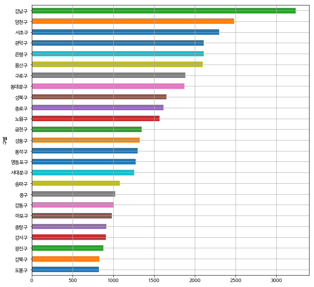
# 구별 CCTV 개수 - 수평 막대 그래프
data_result['소계'].sort_values().plot(kind='barh', grid=True, figsize=(10, 10))
plt.show()
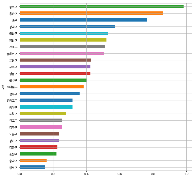
# 인구대비 CCTV비율 시각화 - 수평 막대 그래프
data_result['CCTV비율'] = data_result['소계'] / data_result['인구수'] * 100

data_result['CCTV비율'].sort_values().plot(kind='barh', grid=True, figsize=(10, 10))
plt.show()
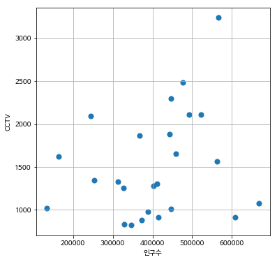
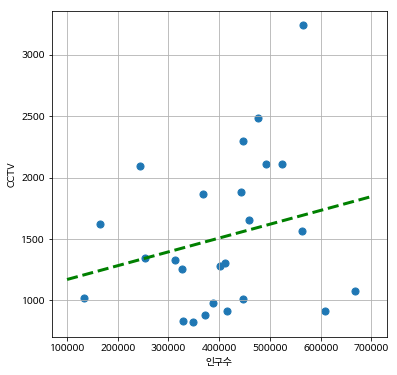
plt.figure(figsize=(6,6))
plt.scatter(data_result['인구수'], data_result['소계'], s=50)
plt.xlabel('인구수')
plt.ylabel('CCTV')
plt.grid()
plt.show()
# linear regression
## 기울기, y절편 구하기
fp1 = np.polyfit( data_result['인구수'], data_result['소계'], 1)
# 직선의 식
f1 = np.poly1d(fp1)
# x축의 범위와 간격 설정
fx = np.linspace(100000, 700000, 100)

# 그래프
plt.figure(figsize=(6,6))
plt.scatter(data_result['인구수'], data_result['소계'], s=50)
# 그래프에 추쇄선 삽입
## ls: line-style,  lw: line-width
plt.plot(fx, f1(fx), ls='dashed', lw=3, color='g')
plt.xlabel('인구수')
plt.ylabel('CCTV')
plt.grid()
plt.show()
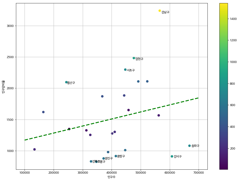
# 경향성에서 벗어난 데이터 찾기
## 기울기, y절편 구하기
fp1 = np.polyfit( data_result['인구수'], data_result['소계'], 1)
## 직선의 식
f1 = np.poly1d(fp1)
## x축의 범위와 간격 설정
fx = np.linspace(100000, 700000, 100)
## 직선과 점 사이의 y축 거리 구하기
data_result['오차'] = np.abs( data_result['소계'] - f1(data_result['인구수']) )
## 오차 순으로 정렬
df_sort = data_result.sort_values(by='오차', ascending=False)
df_sort.head()
| 소계 | 최근증가율 | 인구수 | 한국인 | 외국인 | 고령자 | 외국인비율 | 고령자비율 | CCTV비율 | 오차 | |
|---|---|---|---|---|---|---|---|---|---|---|
| 구별 | ||||||||||
| 강남구 | 3238 | 150.619195 | 565731.0 | 560827.0 | 4904.0 | 64579.0 | 0.866843 | 11.415143 | 0.572357 | 1543.390613 |
| 양천구 | 2482 | 34.671731 | 476627.0 | 472730.0 | 3897.0 | 54598.0 | 0.817620 | 11.455079 | 0.520743 | 887.616126 |
| 강서구 | 911 | 134.793814 | 607877.0 | 601391.0 | 6486.0 | 75046.0 | 1.066992 | 12.345590 | 0.149866 | 831.015839 |
| 용산구 | 2096 | 53.216374 | 243922.0 | 228960.0 | 14962.0 | 36727.0 | 6.133928 | 15.056862 | 0.859291 | 763.366194 |
| 서초구 | 2297 | 63.371266 | 447177.0 | 442833.0 | 4344.0 | 52738.0 | 0.971427 | 11.793540 | 0.513667 | 735.741927 |
# 그래프
plt.figure(figsize=(14, 10))
plt.scatter(data_result['인구수'], data_result['소계'], s=50, c=data_result['오차'])
# 그래프에 추쇄선 삽입
## ls: line-style,  lw: line-width
plt.plot(fx, f1(fx), ls='dashed', lw=3, color='g')

for n in range(10):
    plt.text( df_sort['인구수'][n]*1.01, df_sort['소계'][n]*0.99, df_sort.index[n], fontsize=10  )

plt.xlabel('인구수')
plt.ylabel('인구당비율')
plt.colorbar()
plt.grid()
plt.show()